Predicting Box Office Hits
Posted on Sun 28 February 2016 in articles
Background
Who doesn't like movies? I recently did a data science project where I scraped data from Box Office Mojo, and got to explore some questions I had about the industry.
-
How can adjusted revenue be predicted?
-
Why did some movies flop big time? (I'd bet you've never heard of Mars Needs Moms!)
-
Which movies were surprisingly popular? (Remember The Blair Witch Project!?)
Acquiring Data
Box Office Mojo has data on over 16,000 movies --- buried within a fairly unintuitive and complex layout. This demanded some exploring to figure out the optimal strategy.
After poking around a bit, I found an alphabetical directory which contains links to individual movie pages and other information. I decided to scrape the links and any additional data.
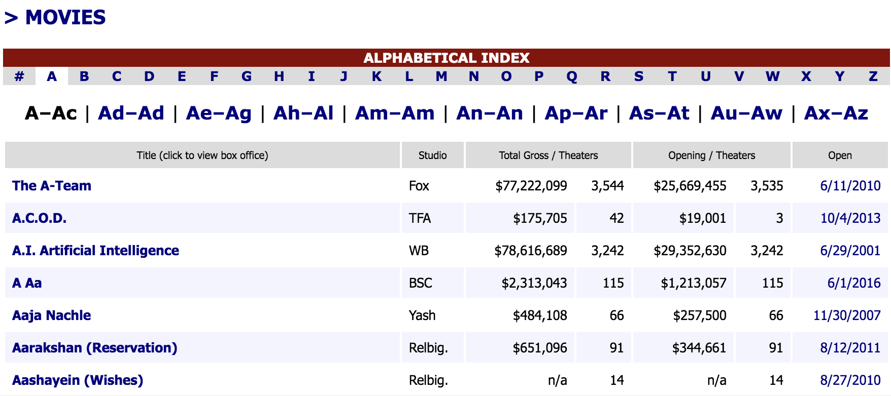
These links allowed me navigate through even more pages -where the true gems were located. Although I wasn't sure everything would be useful, erring on the cautious side seemed wise. Here's a screen shot (this movie brings me back!):
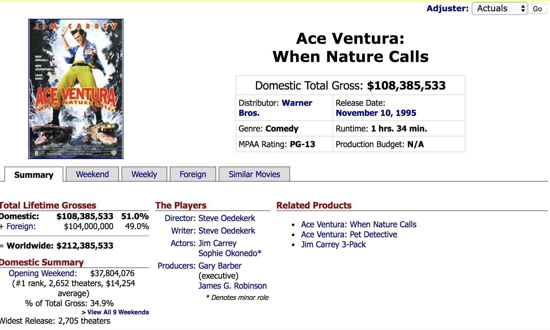
Pandas works very well with nested dictionaries --- I created a Python script to pickle them in preparation for the next steps.
Cleaning
After scraping and loading my data into Pandas, there were several issues which emerged before I could get going on analysis:
-
NA values - After looking into these further, some movies (specifically older ones) didn't have much data. I had to drop these after ensuring there wasn't an error in my scraper.
-
Removing dollar signs, etc.
-
Converting strings to datetime objects or integers - Many values had datatypes which were unsuitable for any statistical analysis, so I had to convert them.
-
Adjusting prices for inflation - I was mindful to use the built-in adjuster when scraping, but I noticed it didn't adjust all prices. I had to adjust other prices for inflation.
After these steps, I was pretty excited to get going on next steps. Whoever said much of data science is not modelling was not joking! I wanted to figure out what is predictive of worldwide revenue.
Exploration
It was helpful to develop some intuition by visualizing variables --- I was curious to see how they related to worldwide revenue.
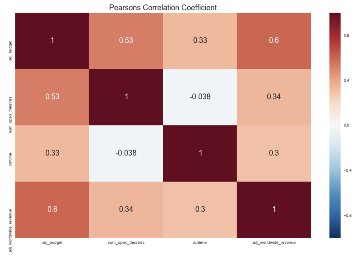
Pandas and seaborn makes this easy and enjoyable (the visualizations are beautiful!) --- below is a heatmap for the correlations of continuous variables.
I also wanted to look into how release month and rating related to worldwide revenue. I really prefer violinplots to barplots or boxplots --- it gives a clearer picture of the distributions.
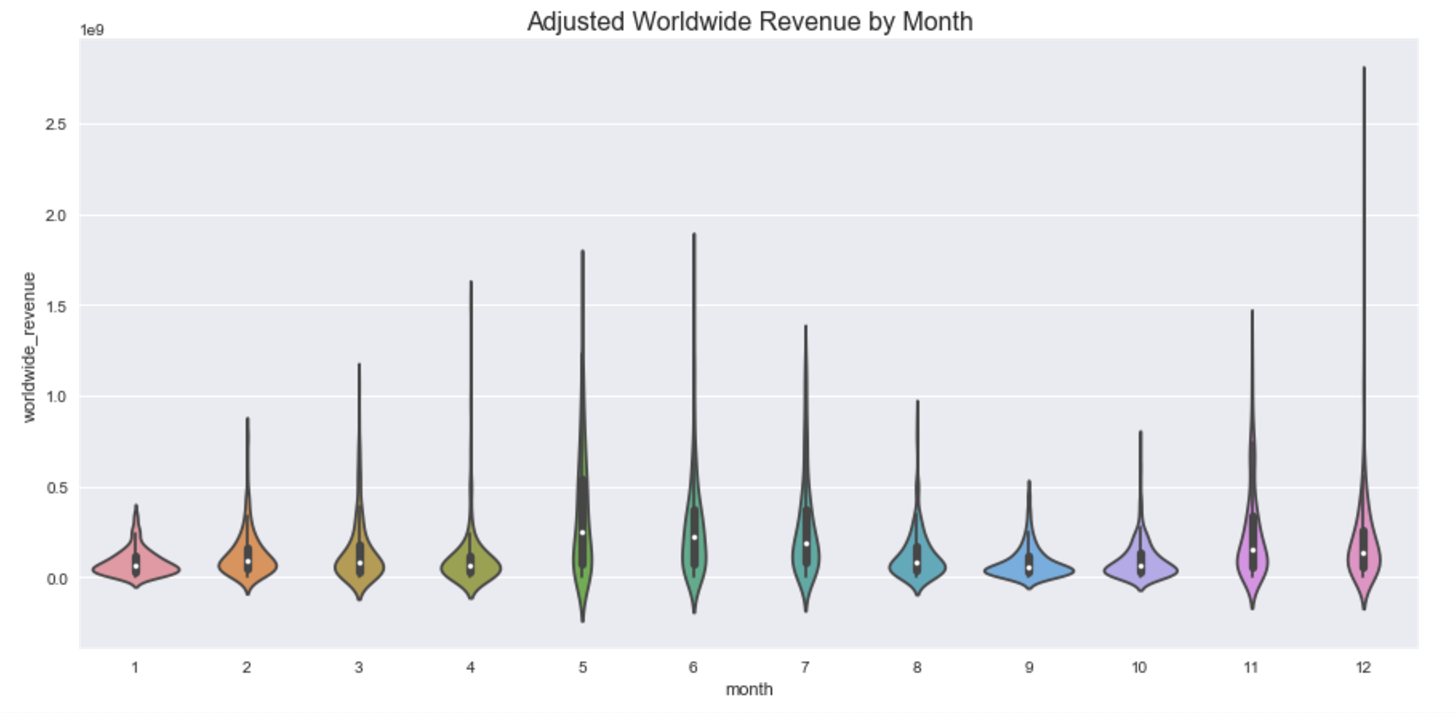
Above we see that adjusted worldwide revenue tends to be larger for months April, May, June, November, and December.
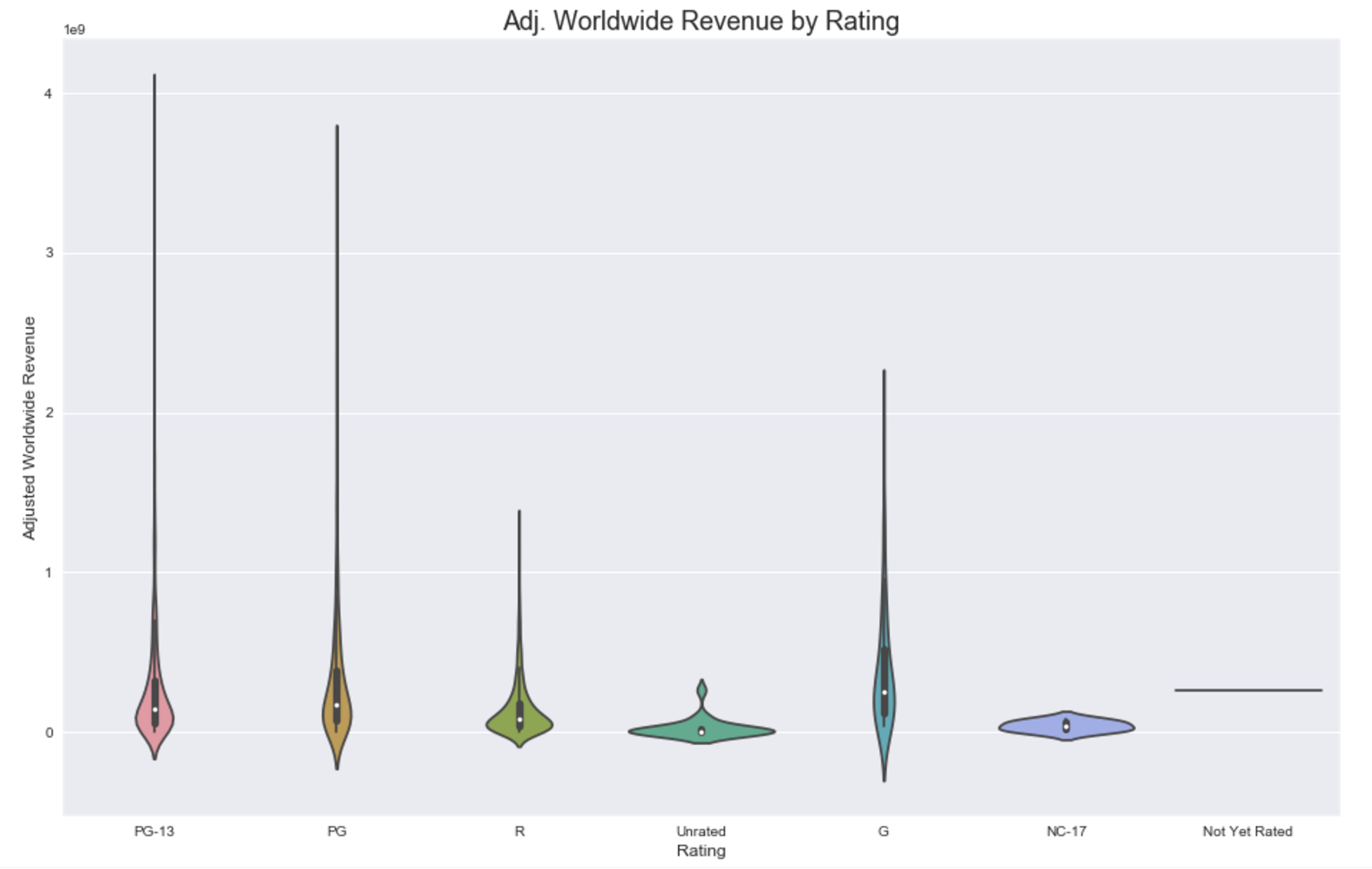
Observe from obove that G rated movies have the highest mean adjusted worldwide revenue, with PG and PG-13 movies varying the most --- and making up a big chunk of the highest AWR.
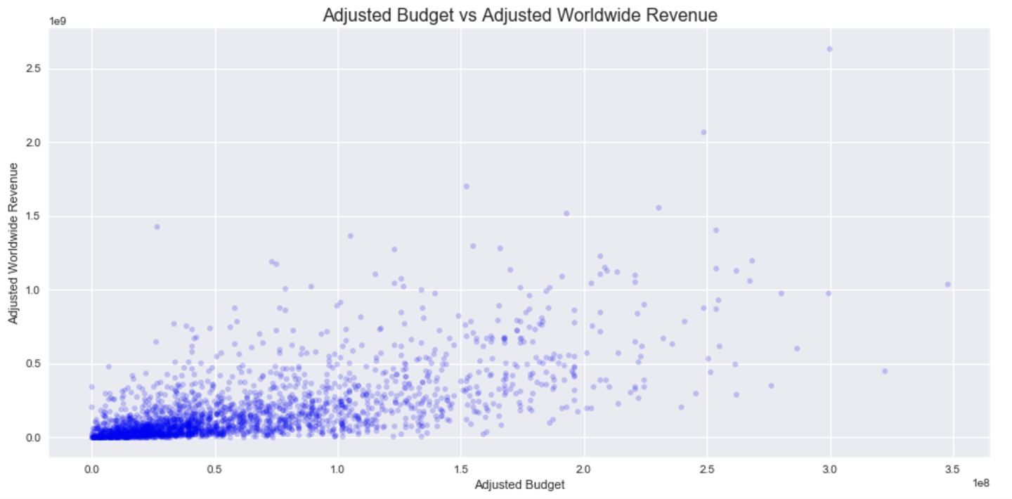
I wanted to continue exploring variables to see if there was a linear relationship between them and adjusted worldwide revenue. I started out with using simple linear regression, formally:
\(y_{i} = \beta_{0} + \beta_{1}x_{i1} + \epsilon_{i}\)
Formally:
\(H_{0}: \beta_{1} = 0\)
\(H_{A}: \beta_{1} \neq 0\)
Below is the simple linear regression for adjusted budget:
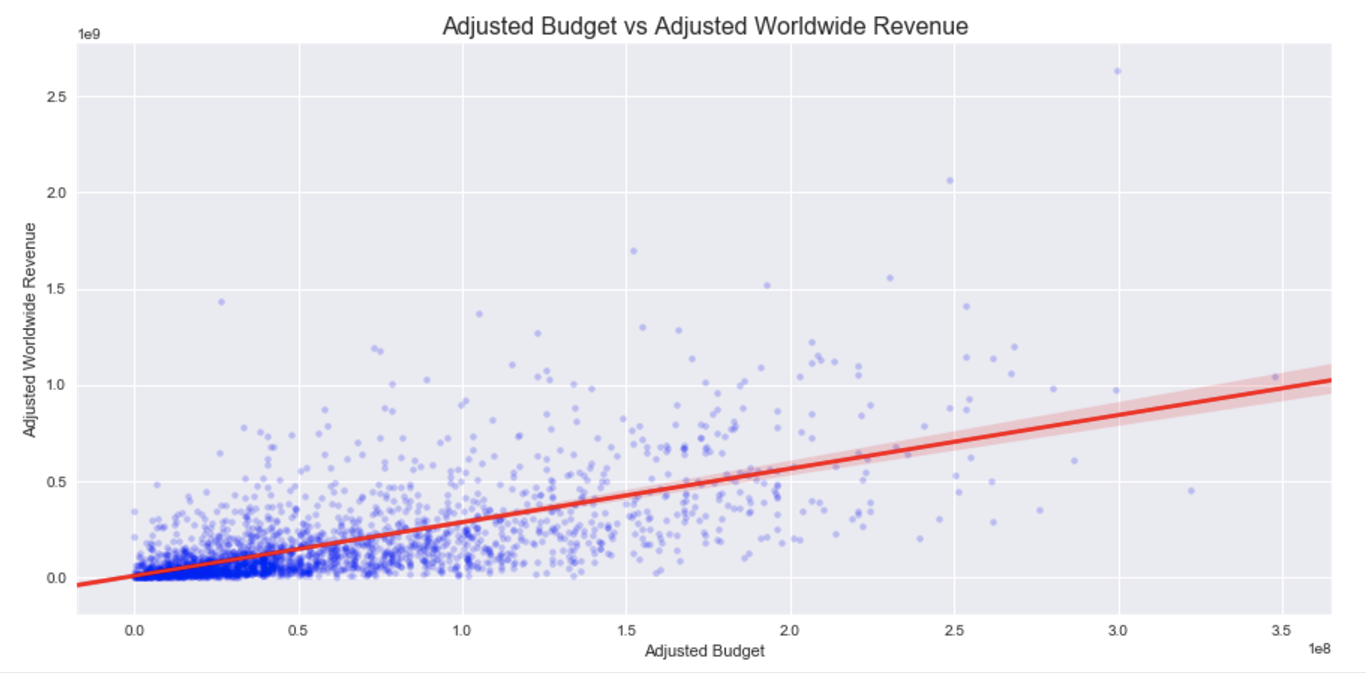
Above, we minimized the residual sum of squares to find our line of best fit, which is the same as maximizing the likelihood of \(\beta_{0}\) and \(beta_{1}\). (There is some interesting discussion about MLE and RSS here.)

The p-value for \(\beta_{1} < .001\) and our 95% CI is (2.658, 2.911), so we can reject \(H_{0}\). Specifically, our initial model has a decent adjusted R-squared of .439 (which is the same as R-squared, in this case). This model can explain nearly 44% of the variance in Adjusted Worldwide Revenue around it's mean - not bad!
However, after analyzing the residuals it is clear our model violates linear regression assumptions - the residuals appear heteroscedastic. There is a glimpse of this because of the cone shape (lighter red in plot above) variance around my regression line. After a closer look, our suspicions are confirmed:
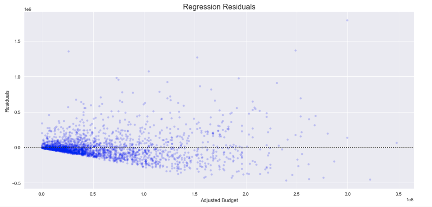
I decided to try a few variable transformations and settled on applying the squareroot to both variables (independent and dependent). The relationships are now more linear. Although there is still slight heteroscedacity, it has greatly improved. In reality, the assumptions of linear regression are rarely perfectly met, but this seems reasonable enough to work with. Checkout the regression plot and residuals below:
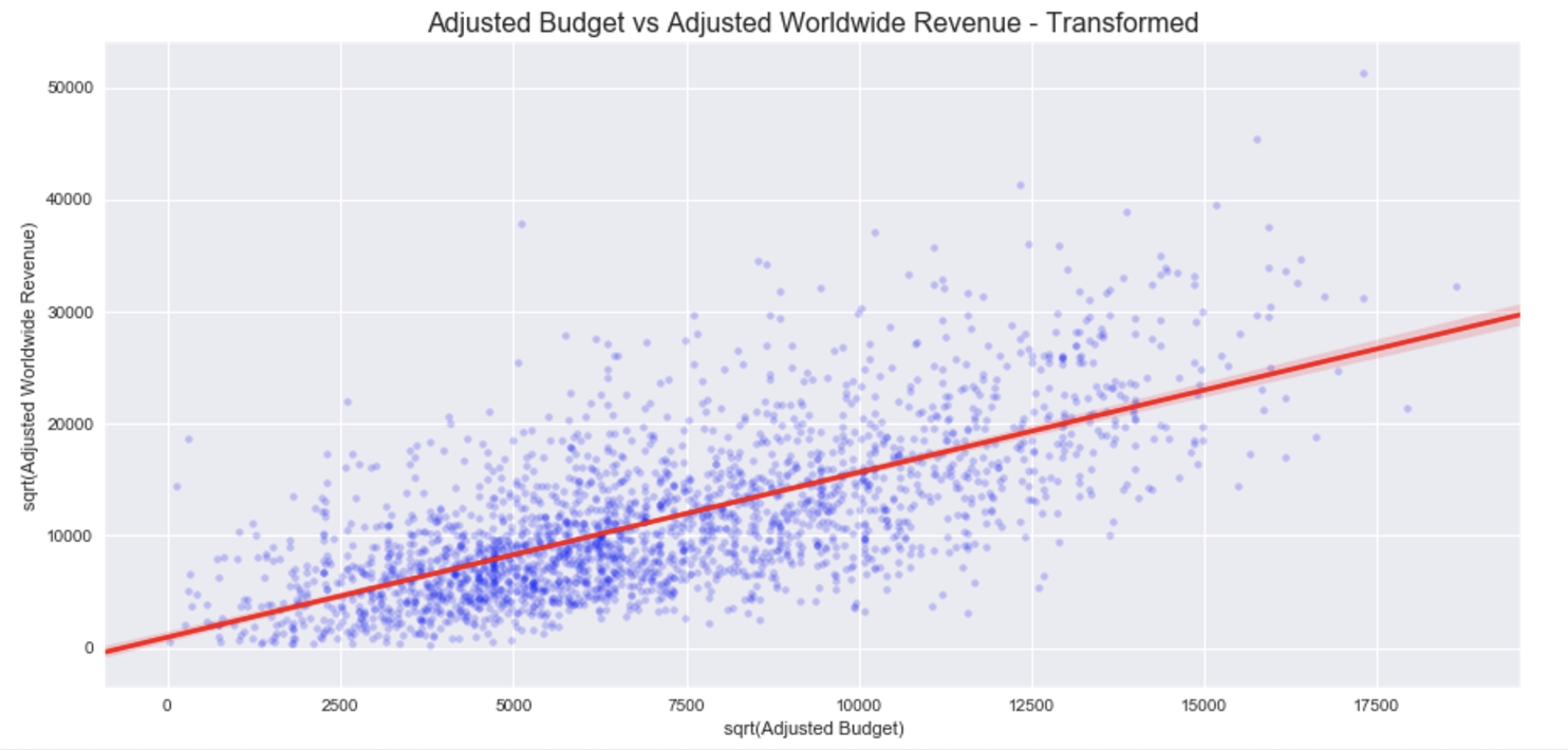
The \(R_{adj}^2\) improved to .478 and p-value remained <.001. Let's keep going!
Further Analysis and Modelling
I continued to explore different variables and evaluate the residuals and regressions. Specifically, I wanted to make sure everything looked normal to evaluate whether I needed to transform variables or had some insights into better features to engineer.
Finally, \(R_{adj}^2\) improved to ~.61 after taking including features for month, number of opening theatres, and runtime. I really liked using Python's statsmodels library because it's great for more statistical purposes with it's reporting tools.
I also wanted to see if our model could explain why 'The Blair Witch Project' was so successful and why 'Mars Needs Moms' flopped so hard. Below are the values for these movies:

'The Blair Witch Project' had nearly 10 times more worldwide revenue, despite having a lower runtime, less opening theatres, and a far lower budget than 'Mars Needs Moms'. However, I think the timing for the BWP was especially important - releasing a movie targeting teens and young adults near popular months could be a recipe for the viral movie it was.
After looking a little closer, the BWP was released in early July - when the target audience had summer break from school. I'm hesitant to delve any deeper into the emotional appeal of either film, but it'd be interesting to see how prevalent viral films are in popular months.
After this, I wanted to move to Sci-kit learn because it has more optionality when it comes to tuning hyper parameters using cross validation tools. Time to jump in!

Final Model and Validation
I wanted to check out the cross validation tools in sci-kit learn (does anyone say Sklearn?) so I experimented with Lasso (L1) and Ridge (L2) regularization, but ultimately settled on ElasticNet (which uses both).
The ElasticNetCV module is extremely powerful - it will perform K-Fold cross validation and choose the best parameters for you.
After training my model on 2/3 of the data using K-Fold ElasticNetCV, it performed well on the unseen data with \(R_{adj}^2\) ~ .65 which wasn't too bad!
What I Learned
Although it could have been faster to automate building the model, I really learned a lot by going step-by-step and evaluating it myself. It was also really helpful to develop an understanding of the data beforehand.
I also learned how to webscrape and handle a plethora of inevitable errors. BeautifulSoup was pretty time consuming, - I would like to try out Selenium in the future to see how it compares.
Although I certainly learned a lot, there are definitely things I'd do further.

Further Steps
There are more economic indicators and data available about the entertainment industry. It would also be interesting to look further into trends and seasonal effects. Also, it would be interesting to analyze social media or wikipedia.
If I had more time, there are a lot more things I'd like to take a look (or closer look!) into. There is so much data publicly available that it wouldn't be too difficult to supplement my dataset with economic, entertainment, and social data. Furthermore, I'd like to take a closer look at trends and seasonality.
Additionally, I'd optimize and more thoroughly test my code, and even automate a lot of the modelling. I think that would save a lot of time and possibly even be re-usable for other projects.
I really enjoyed this project - I thought it was a good overall view of the data science process. Ultimately, data scraping can be an extremely useful tool --- not every dataset is nice and neat like in academia or kaggle.